Originally: April 3, 2016 (Updated January 24, 2022)
Executive Summary: Who in NYC would benefit from an Earned Income Tax Credit expanded to filers without dependents? This analysis of the New York City Center for Economic Opportunity’s 2013 data set offers a better understanding of which residents are in need of a wider EITC and why. The report verifies the CEO’s methodology for estimating NYC poverty rates and demonstrates that the rate is actually higher at the individual level. Additionally the report looks at leading causes of extremely low and high incomes observed under the CEO’s unique poverty measure, highlighting the advantages of the NYC CEO’s measure of poverty over the nationwide measure. Finally an in-depth demographic statistical analysis is conducted to better understand who still ends up below the poverty line well after Federal benefits are accounted for.
Those who remain in poverty are significantly more likely than the general population to be Black and Latino, live in the Bronx and Brooklyn, and be socioeconomically vulnerable. Surprisingly in comparison to the whole poor population those not lifted above the poverty line after benefits are more likely to be White and Asian and hold a HS education or more. The results suggest that this population may be particularly concentrated with students or recent college graduates, although further research is necessary.
Introduction:
Data for this analysis was accessed from New York City’s Economic Opportunity website originally on March 3, 2016 (updated January 24, 2022) at this address: https://www1.nyc.gov/site/opportunity/poverty-in-nyc/poverty-data.page
The CEO’s survey data set includes variables from the Census Bureau’s American Community Survey alongside the CEO’s own variables. There are a total of 66950 respondants across 539 variables.
January 2022 update: The housing status variable is either incorrectly named or missing from the most recent version of the dataset.
Data Munging:
library(plyr)
filename <- "2013 NYC Web Dataset.csv"
`2013.NYC.ACS.CEO` <- read.csv(filename)
# Doing some data munging now. Going to code certain variables that will be important to later demographic analysis.
# January 2022 Update: Housing Status codes will be commented out.

`2013.NYC.ACS.CEO`$Boro = as.character(`2013.NYC.ACS.CEO`$Boro)
#`2013.NYC.ACS.CEO`$EST_HousingStatus = as.character(`2013.NYC.ACS.CEO`$EST_HousingStatus)
`2013.NYC.ACS.CEO`$Ethnicity = as.character(`2013.NYC.ACS.CEO`$Ethnicity)
`2013.NYC.ACS.CEO`$EducAttain = as.character(`2013.NYC.ACS.CEO`$EducAttain)
`2013.NYC.ACS.CEO`$CitizenStatus = as.character(`2013.NYC.ACS.CEO`$CitizenStatus)
`2013.NYC.ACS.CEO`$FTPTWork = as.character(`2013.NYC.ACS.CEO`$FTPTWork)

`2013.NYC.ACS.CEO`$Boro[`2013.NYC.ACS.CEO`$Boro == 1] = "Bronx"
`2013.NYC.ACS.CEO`$Boro[`2013.NYC.ACS.CEO`$Boro == 2] = "Brooklyn"
`2013.NYC.ACS.CEO`$Boro[`2013.NYC.ACS.CEO`$Boro == 3] = "Manhattan"
`2013.NYC.ACS.CEO`$Boro[`2013.NYC.ACS.CEO`$Boro == 4] = "Queens"
`2013.NYC.ACS.CEO`$Boro[`2013.NYC.ACS.CEO`$Boro == 5] = "Staten Island"

#`2013.NYC.ACS.CEO`$EST_HousingStatus[`2013.NYC.ACS.CEO`$EST_HousingStatus == 1] = "Public Housing"
#`2013.NYC.ACS.CEO`$EST_HousingStatus[`2013.NYC.ACS.CEO`$EST_HousingStatus == 2] = "Mitchell Lama"
#`2013.NYC.ACS.CEO`$EST_HousingStatus[`2013.NYC.ACS.CEO`$EST_HousingStatus == 3] = "Subsidized"
#`2013.NYC.ACS.CEO`$EST_HousingStatus[`2013.NYC.ACS.CEO`$EST_HousingStatus == 4] = "Rent Regulated"
#`2013.NYC.ACS.CEO`$EST_HousingStatus[`2013.NYC.ACS.CEO`$EST_HousingStatus == 5] = "Other Regulated"
#`2013.NYC.ACS.CEO`$EST_HousingStatus[`2013.NYC.ACS.CEO`$EST_HousingStatus == 6] = "Market"
#`2013.NYC.ACS.CEO`$EST_HousingStatus[`2013.NYC.ACS.CEO`$EST_HousingStatus == 7] = "No Cash"
#`2013.NYC.ACS.CEO`$EST_HousingStatus[`2013.NYC.ACS.CEO`$EST_HousingStatus == 8] = "Fully Owned"
#`2013.NYC.ACS.CEO`$EST_HousingStatus[`2013.NYC.ACS.CEO`$EST_HousingStatus == 9] = "Owned Mortgage"
#`2013.NYC.ACS.CEO`$EST_HousingStatus[`2013.NYC.ACS.CEO`$EST_HousingStatus == 10] = "Non-building Housing" # New code.

`2013.NYC.ACS.CEO`$Ethnicity[`2013.NYC.ACS.CEO`$Ethnicity == 1] = "White"
`2013.NYC.ACS.CEO`$Ethnicity[`2013.NYC.ACS.CEO`$Ethnicity == 2] = "Black"
`2013.NYC.ACS.CEO`$Ethnicity[`2013.NYC.ACS.CEO`$Ethnicity == 3] = "Asian"
`2013.NYC.ACS.CEO`$Ethnicity[`2013.NYC.ACS.CEO`$Ethnicity == 4] = "Hispanic"
`2013.NYC.ACS.CEO`$Ethnicity[`2013.NYC.ACS.CEO`$Ethnicity == 5] = "Other"

`2013.NYC.ACS.CEO`$EducAttain[`2013.NYC.ACS.CEO`$EducAttain == 1] = "No HS"
`2013.NYC.ACS.CEO`$EducAttain[`2013.NYC.ACS.CEO`$EducAttain == 2] = "HS"
`2013.NYC.ACS.CEO`$EducAttain[`2013.NYC.ACS.CEO`$EducAttain == 3] = "Some College"
`2013.NYC.ACS.CEO`$EducAttain[`2013.NYC.ACS.CEO`$EducAttain == 4] = "College or More"

`2013.NYC.ACS.CEO`$CitizenStatus[`2013.NYC.ACS.CEO`$CitizenStatus == 1] = "Citizen By Birth"
`2013.NYC.ACS.CEO`$CitizenStatus[`2013.NYC.ACS.CEO`$CitizenStatus == 2] = "Naturalized"
`2013.NYC.ACS.CEO`$CitizenStatus[`2013.NYC.ACS.CEO`$CitizenStatus == 3] = "Not A Citizen"

`2013.NYC.ACS.CEO`$FTPTWork[`2013.NYC.ACS.CEO`$FTPTWork == 1] = "Full Time"
`2013.NYC.ACS.CEO`$FTPTWork[`2013.NYC.ACS.CEO`$FTPTWork == 2] = "Part Time"
`2013.NYC.ACS.CEO`$FTPTWork[`2013.NYC.ACS.CEO`$FTPTWork == 3] = "No Work"

`2013.NYC.ACS.CEO`$EducAttain[`2013.NYC.ACS.CEO`$Povrel == 1] = "Head"
`2013.NYC.ACS.CEO`$EducAttain[`2013.NYC.ACS.CEO`$Povrel == 2] = "Spouse/Partner"
`2013.NYC.ACS.CEO`$EducAttain[`2013.NYC.ACS.CEO`$Povrel == 3] = "Child"
`2013.NYC.ACS.CEO`$EducAttain[`2013.NYC.ACS.CEO`$Povrel == 4] = "Other"

# Creating variables that are aggregates of the data for later analysis on the Poverty Unit level.
CEOIncPov = cbind.data.frame(`2013.NYC.ACS.CEO`$SERIALNO, `2013.NYC.ACS.CEO`$NYCgov_Income, `2013.NYC.ACS.CEO`$NYCgov_Threshold, `2013.NYC.ACS.CEO`$NYCgov_Pov_Stat, `2013.NYC.ACS.CEO`$Off_Pov_Stat, `2013.NYC.ACS.CEO`$PreTaxIncome_PU, `2013.NYC.ACS.CEO`$Off_Threshold, `2013.NYC.ACS.CEO`$EST_Housing, `2013.NYC.ACS.CEO`$EST_Childcare, `2013.NYC.ACS.CEO`$EST_Commuting, `2013.NYC.ACS.CEO`$EST_MOOP, `2013.NYC.ACS.CEO`$EST_HEAP, `2013.NYC.ACS.CEO`$EST_Nutrition, `2013.NYC.ACS.CEO`$Povunit_ID)

# These variable names are very long. Let's make them more succinct.

colnames(CEOIncPov) = c("IncPovSerial", "CEO_Inc", "CEO_Thresh", "Poor", "Off_Poor", "Pretax", "Off_Thresh", "Housing", "Childcare", "Commuting", "MOOP", "HEAP", "Nutrition", "Pov_Unit")

# Now let's make variables of subsetted poor and safe Poverty Units (roughly households).

SimpCEOPoor = subset(CEOIncPov, Poor == 1)
SimpCEOSafe = subset(CEOIncPov, Poor == 2)

# Aggregating these subsets so we can look at Poverty Unit (household) level data!

AggSimpCEOPoor = aggregate(cbind(CEO_Inc, CEO_Thresh, Poor, Off_Poor, Pretax, Off_Thresh, Housing, Childcare, Commuting, MOOP, HEAP, Nutrition, Pov_Unit)~IncPovSerial, data=SimpCEOPoor, FUN=mean)

AggSimpCEOSafe = aggregate(cbind(CEO_Inc, CEO_Thresh, Poor, Off_Poor, Pretax, Off_Thresh, Housing, Childcare, Commuting, MOOP, HEAP, Nutrition, Pov_Unit)~IncPovSerial, data=SimpCEOSafe, FUN=mean)
Analysis: Question 1: By the CEO’s classification, what was the poverty rate in New York City in 2013? Is there more than one way to estimate it?
Accepting the CEO’s survey sample as representative of the City, a look at the observed proportion of people classified as poor versus not poor by the CEO’s measure theoretically should provide the poverty rate.
The CEO’s measure is being used because it is more applicable to the cost of living in NYC than the US Census Bureau’s measure of poverty, which does not have a mechanism to account for some costs of living.
Povtable = table(`2013.NYC.ACS.CEO`$NYCgov_Pov_Stat)
Povrate = Povtable[1]/Povtable[2]
Povrate
## 1
## 0.2364946The City’s estimated poverty rate in 2013 was 25.2% by this calculation. It is higher than the 23.6% the CEO reports because this measure rawly accounted for individual poverty rates. The CEO on the other hand specifically uses “poverty units.” The definition of that can be obtained in Appendix A of the latest CEO Poverty Measure report here: http://www.nyc.gov/html/ceo/downloads/pdf/NYCgov_Pov_Stat_measure_2005_2013.pdf
Regardless the CEO’s measure of poverty can be obtained with some data transformation.
# Using the column "Povunit" in the 2013 data set allows us to arrive at a total of all the units in the survey and use the "Poor"/"Not Poor" classification of those units to arrive at the CEO's poverty rate.

# Let's break our data set up into respondents classified as "Poor" or "Not Poor".

CEOPoor = subset(`2013.NYC.ACS.CEO`, NYCgov_Pov_Stat == 1)
CEOSafe = subset(`2013.NYC.ACS.CEO`, NYCgov_Pov_Stat == 2)
SafeUnits = sum(CEOSafe$Povunit_ID) # The number of not poor units in our survey.
PoorUnits = sum(CEOPoor$Povunit_ID) # The number of poor units in our survey.
CEOPovRate = PoorUnits/(PoorUnits + SafeUnits)
CEOPovRate
## [1] 0.2041013To paraphrase the Center of Economic Opportunity, this method of reaching the poverty rate effectively excludes those who reasonably wouldn’t be expected to generate an income. Some of the analysis later may show why this assumption could be dangerous.
Question 2: What’s the highest and lowest observed “CEO Income” under the CEO Poverty Threshold in 2013?
min(CEOPoor$NYCgov_Income)## [1] -25999.36The above was included to demonstrate a flaw of looking at just the minimum value in the data set.
Since each respondent in a household is given a row on the survey the same household may seem to “repeat” multiple times in the dataset. To address this the responses were aggregated by their ACS-given household serial number and include some of the vital CEO variables.
The CEO income is adjusted to account for government benefits and housing, childcare, commuting, and medical expenses. Without that context the figure $-25,999 might seem like an alarming mistake. A look at that response line gives a better idea of how this figure was calculated.
MinPoor = AggSimpCEOPoor[which(AggSimpCEOPoor$CEO_Inc == min(AggSimpCEOPoor$CEO_Inc)),]
MinPoor[c("CEO_Inc", "Pretax", "Housing", "Childcare", "Commuting", "Nutrition", "HEAP", "Off_Thresh")]
ResultMinPoor = MinPoor["Pretax"] - MinPoor["Housing"] - MinPoor["Childcare"] - MinPoor["Commuting"] + MinPoor["Nutrition"] + MinPoor["HEAP"]
ResultMinPoorThe above verifies that the minimum CEO income figure is the result of a household with a very low pre-tax income ($14,405.45) and burdened by an extraordinary out-of-pocket Medical debt ($117,857.70) that is hardly off-set by limited Food Stamps ($4,404) and Home Energy Assistance ($25).
The minimum income in this dataset is espcially notable because based solely on this respondent’s pre-tax income they are above the official nationwide poverty threshold.
Now to look at the highest income under the CEO poverty line.
MaxPoor = AggSimpCEOPoor[which(AggSimpCEOPoor$CEO_Inc == max(AggSimpCEOPoor$CEO_Inc)),]
MaxPoor[c("CEO_Inc", "CEO_Thresh", "Pretax", "Off_Thresh", "MOOP", "Housing", "Commuting", "Nutrition", "HEAP", "Pov_Unit")]
Question 3: Which New Yorkers were brought above the nationwide poverty line after accounting for the benefits and costs the CEO measures?
Considering how vital benefits, or the lack of an adequate amount of them, have been to the previous questions it seems pertinent to get an idea of what proportion of the poor were brought out of poverty (at least by the US’ measurement) after benefits and costs considered by the CEO.
# Taking the total number of surveyed New Yorkers who no longer qualify as poor by nationwide standards and divide that number by the count of all of those who qualified.

Official.Pov = rbind(subset(AggSimpCEOPoor, Off_Poor == 1), subset(AggSimpCEOSafe, Off_Poor == 1))

Rescued.Off.Pov = subset(Official.Pov, CEO_Inc > Off_Thresh)

nrow(Rescued.Off.Pov)/nrow(Official.Pov)
## [1] 0.4186693About 42% of poor New Yorkers were brought above the national poverty line after accounting for benefits and costs the CEO typically measures.
Medical expenses can be a huge source of debt for many families. How much higher would our rescued rate have been if these families had no medical expenses?
HRescued.Off.Pov = subset(Official.Pov, CEO_Inc+MOOP > Off_Thresh) # The same variable as above, except with Medical Out Of Pocket Expenses added back into the CEO's reported income.
nrow(HRescued.Off.Pov)/nrow(Official.Pov)
## [1] 0.4631579The figure jumps to over 46% once medical expenses are handled. Some statistical analysis can tell us what the demographics are of the 60% who aren’t lifted out of poverty by these benefits.
Indi.Off.Pov = subset(`2013.NYC.ACS.CEO`, Off_Pov_Stat == 1) # We need to capture individual level data for this part of the analysis, so we're back to pulling data from the original frame - no aggregation.
NoRescued.Off.Pov = subset(Indi.Off.Pov, NYCgov_Income+EST_MOOP+EST_Commuting < Off_Threshold) # Let's leave large Medical Expenses and Commuting expenses out of the analysis. We'll keep other expenses because some benefits are meant to offset those anyway.
Indi.Rescued.Off.Pov = subset(Indi.Off.Pov, NYCgov_Income+EST_MOOP+EST_Commuting > Off_Threshold)
#ChronPoorDemos = table(NoRescued.Off.Pov$Boro, NoRescued.Off.Pov$EST_HousingStatus, NoRescued.Off.Pov$Ethnicity)
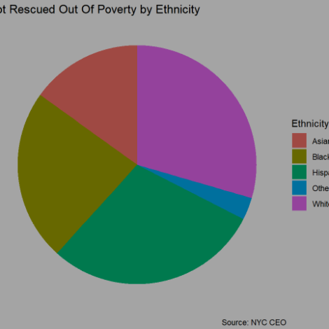
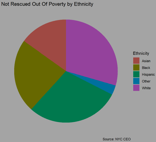
ChronPoorDemos = table(NoRescued.Off.Pov$Boro, NoRescued.Off.Pov$Ethnicity)
SumsOfChronPoor = addmargins(ChronPoorDemos, FUN=sum)## Margins computed over dimensions
## in the following order:
## 1:
## 2:SumsOfChronPoor##
## Asian Black Hispanic Other White sum
## Bronx 36 260 591 27 82 996
## Brooklyn 238 634 384 52 700 2008
## Manhattan 88 109 156 16 230 599
## Queens 360 219 354 71 324 1328
## Staten Island 24 25 57 3 113 222
## sum 746 1247 1542 169 1449 5153The above table gives an example of some demographic distributions among the poverty stranded individuals.
# Now we'll check to see if the distribution of some of these attributes is significantly different from distribution of the rest of the surveyed respondents. Race will be the example here of how this analysis is done, but each analysis run on these traits can be found in the accompanying script.

ObsRaceDist = c(867, 1306, 1612, 168, 1578) # The racial distribution of those not lifted by benefits.
PopRaceDist = c(9858, 14425, 16283, 1962, 24422)/66950 # The racial proportions of the survey respondents.

chisq.test(ObsRaceDist,p=PopRaceDist)
##
## Chi-squared test for given probabilities
##
## data: ObsRaceDist
## X-squared = 163.27, df = 4, p-value < 2.2e-16# The low p-value suggests that there is a statistically significant difference in the racial distribution of those not lifted by the benefits programs.
table(`2013.NYC.ACS.CEO`$Ethnicity)/nrow(`2013.NYC.ACS.CEO`)##
## Asian Black Hispanic Other White
## 0.14724421 0.21545930 0.24321135 0.02930545 0.36477969table(NoRescued.Off.Pov$Ethnicity)/nrow(NoRescued.Off.Pov)##
## Asian Black Hispanic Other White
## 0.14477004 0.24199495 0.29924316 0.03279643 0.28119542Based on the table it’s clear that a disproportionate number of Black and Latino respondents remained below the official poverty line even after accounting for benefits. On the other hand the opposite could be said for White respondents.
After repeating this process for other variables a profile was sculpted from which was built a model of the respondent least likely to be raised above the poverty line by benefit programs alone. Those respondents are significantly more likely than all surveyed to be Black and Latino, renting in the Bronx and Brooklyn without citizenship. Actually, they’re highly likely to be living in subsidized, regulated, market rate, and Mitchell Lama housing. These respondents are more likely to have terminated their education at or before completing high school and are far less likely to hold full time employment year round.
Even among the poor those stuck at the bottom posses significantly different demographic characteristics. For example, they are more likely to be Asian or White, less likely to be Latino, and still overrepresented in the Bronx and Brooklyn, while underrepresented in Queens and Staten Island. Noticably they’re also less likely than the whole poor population to have achieved anything less than a HS diploma.
Is the average income of people stuck at the bottom significantly different from those of everyone below the official poverty line?
# A t-test to answer statistically if the incomes of those stranded in poverty are significantly different.

meanTtest = function(x, m, s, n){ # x = observed mean of sample, m = estimated mean of the population,s = standard error, n = number of observations
t = (x - m)/(s/sqrt(n))
DoT = pt(t, df=n-1) # DoT = Distribution function of T
return(DoT)
}

sd(NoRescued.Off.Pov$PreTaxIncome_PU) # SD is huge. Checking next summary statistics of this data.
## [1] 5884.784summary(NoRescued.Off.Pov$PreTaxIncome_PU)## Min. 1st Qu. Median Mean 3rd Qu. Max.
## -5340.0 503.8 5037.7 6091.6 9672.5 35969.5boxplot(NoRescued.Off.Pov$PreTaxIncome_PU) # Looks like many outliers potentially above $25,000 income line according to the box plot. Outliers could bias our standard error estimate, they need to be removed for an accurate t-test.
NoOutsNoResOffPov = subset(NoRescued.Off.Pov, PreTaxIncome_PU < 25000) # Gets rid of a majority of the outliers

OPM = mean(Indi.Off.Pov$PreTaxIncome_PU) # Comparing individuals.
ROPM = mean(Indi.Rescued.Off.Pov$PreTaxIncome_PU)
x = mean(NoOutsNoResOffPov$PreTaxIncome_PU)
s = sd(NoOutsNoResOffPov$PreTaxIncome_PU)
n = nrow(NoOutsNoResOffPov)
meanTtest(x = x, m = OPM, s = s, n = n) # Testing the observed mean against the mean of all individuals under the official poverty line.
## [1] 0meanTtest(x = x, m = ROPM, s = s, n = n) # Testing the observed mean against the mean of individuals below the poverty line who were rescued by benefits programs.## [1] 0The p values of these t-tests confirm that those remaining below the poverty line, even after benefits, earned significantly less pre-tax income on average than the general poor population ($6357 versus $12065).
The total size of the benefits recieved may be a contributing factor to how mobile respondent become. Such a hypothesis can be statistically tested.
# The following will test if the average benefits package of residents without post-benefits mobility is significantly different from the average benefits package given to the poor who get lifted.

MeanBenefitsRes = sum(mean(Indi.Rescued.Off.Pov$EST_HEAP), mean(Indi.Rescued.Off.Pov$EST_Nutrition))
MeanBenefitsNoRes = sum(mean(NoOutsNoResOffPov$EST_HEAP), mean(NoOutsNoResOffPov$EST_Nutrition))

MeanBenefitsRes # Average Benefits for individuals lifted above the poverty line by benefits.
## [1] 5438.766MeanBenefitsNoRes # Average benefits for individuals kept below the poverty line after benefits.## [1] 2790.023EstMeanVar = sum(var(NoOutsNoResOffPov$EST_HEAP), var(NoOutsNoResOffPov$EST_Nutrition))
SDBenefitsNoRes = sqrt(EstMeanVar/5)
# Took the square root of the average variance of all the benefits to estimate the standard error.
meanTtest(x=MeanBenefitsNoRes, m=MeanBenefitsRes, s=SDBenefitsNoRes, n=n)## [1] 0The nearly $3,000 difference in benefits between both mobile and stagnant subsets is statistically significant.
Discussion, Conclusion, and Further Research:
While 1 in 5 New York households are below the CEO’s poverty line fully 1 in 4 New Yorkers qualify as impoverished by the same standards. That difference is relevant when looking at who’s chronically below the poverty line even after recieving federal benefits: educated heads of households and many non-citizens, who make low wages and live in the poorest boroughs.
Medical expenses can pose a huge burden for many, as exmplified by the respondent with the lowest CEO-adjusted income analyzed above. Healthcare costs are known to be the leading cause of bankruptcy in the United States, a fact reinforced by a February 2006 study published in Health Affairs. This is certainly a large part of why NYC’s Center for Economic Opportunity takes those costs into account for its poverty rate considerations.
Using the minimum observed income as a case study additionally highlights the need for an adjusted assessment of poverty in New York City. Even before medical costs were considered, the respondents’ pre-tax income placed the household below the CEO’s poverty threshold but above the national one.
On the other end of the spectrum, why were the benefits distributed to the highest CEO-poor household so high? The household’s Poverty Unit type variable should be noted. “1” is used to designate poverty units consisting of a Husband/Wife and child. Such large households gained from generous food stamp (SNAP) benefits after a Congressional hike in 2009. Unfortunately the recent cuts in SNAP benefits from 2015 put households like these in danger of falling below the CEO and official poverty line again.
But as the analysis demonstrated the households most in danger of not getting up after the fall may be the smallest. The gap between the size of their benefits packages and those of poor mobile respondents is potentially why this segment of New Yorkers remain below the poverty line.
These insights support the theory that having more individuals identifying as heads of the household and fewer “children” or other dependents in a sample contributes to reducing benefit amounts. Many programs, especially SNAP (Food Stamp), School Lunch, and School Breakfast programs will provide households more benefits if they have more dependents.
These results regarding who’s stuck at the bottom exemplify one of today’s pivotal public policy questions: should benefit programs and the Earned Income Tax Credit (EITC) be further expanded for individuals without dependents? There’s a strong case here: many of those falling through the cracks in the current system are in a position for social mobility, attaining educational goals beyond the rest of the impoverished population. But they’re also more likely to be non-citizens living in the City’s poorest counties. Additionally their low incomes despite holding diplomas and degrees could signal that either many of them are current and recent students or that their credentials don’t hold as much value as those enjoyed by others.
Further research should be conducted into the demographics of this subset, especially into their educational attainments and long-term socioeconomic mobility.