
Executive Summary:
Predicting crime, and in particular violent crime, has a long history in the literature of many social sciences. And for good reason, as crime rates have been of practical interest to the American public since at least 1870. Typically linear regression models would be estimated to predict a continuous numerical variable like crime rates. More recently though computer algorithms, especially machine learning models, have been researched as a way to predict crime in the US. This analysis compares an ordinary least squares estimated linear regression model to five machine learning models on their ability to predict violent crime rates in the US using variables from the US Census. The linear regression model was competitive with the non-ensemble method machine learning models, but surpassed by the GLM Boosting and Random Forest models. This suggests that the high variability in the dataset, likely due to correlations between racial concentration, family structure, and violent crime is best handled by ensemble models that improve upon weak base learner models.
Introduction:
Predicting crime rates is probably a hope as old as measuring crime. According to a 1977 publication by Michael Maltz, an Associate Professor at the University of Illinois at Chicago Circle, Congress brought Federal attention to crime reporting in June of 1870 when they passed PL 41-97. The law established the Department of Justice and an obligation for the US Attorney General to report national crime statistics to Congress. The law was mostly ignored until sentiments that crime was rising in the 1920s and 30s led Congress in June of 1930 to task the Federal Bureau of Investigation (FBI) with collecting and disseminating crime statistics. Earlier that year the International Association of Chiefs of Police alongside the Social Science Research Council had published the first version of what we know today as the FBI’s Uniform Crime Report.
There is a rich history of crime prediction approaches in the literature. More recently researchers have advocated the benefits of applying machine learning models to predicting crime rates.
This analysis relies heavily on the 1995 US FBI Uniform Crime Report, as well as the 1990 US Census and the 1990 US Law Enforcement Management and Administrative Statistics Survey. This same dataset was used by Redmond and Highley in 2010 to apply Case-Editing approaches to predicting violent crime rates. Violent Crime Per Person is predicted for 443 jurisdictions using six models, including ordinary least squares linear regression and machine learning algorithms. The models are evaluated based on the R-squared and Root Mean Squared Errors of their predictions.
Data Materials
The analyzed dataset was donated by Michael Redmond of LaSalle University and can be downloaded here. Within are 123 potential predictor variables obtained from the 1990 US Census and the 1990 US Law Enforcement Management and Administrative Statistics Survey. There are 17 additional dependent variables, including values for violent crime per person in most of the 2215 jurisdictions aggregated.
Six models were trained against 1597 (80% of the dataset) randomly selected jurisdictions with recorded violent crime rates and used to predict Violent Crime per person in the remaining 442 jurisdictions.
Violent crime rates are not normally distributed based on the Shapiro-Wilk normality test. Rates average about 589 per person with a standard deviation of 614 per person and a midpoint value of about 374 per person.

In pre-processing, independent variables with missing observations were dropped. Afterward 101 independent variables were left for the analysis. For all the regression models, the dataset was shuffled and split into two sets: training set and validation set. 20% of the data were held for validation, and 80% of the data were used for training. Tenfold cross-validation was applied to the training set for the K-Nearest Neighbor and Support Vector Machines models.
For the KNN models the independent variable values were scaled to a mean of 0 and a standard deviation of 1.
Ordinary Least Squares Linear Regression
A linear regression model was specified, iteratively built with predictor covariances as a starting point for selecting independent variables. Variables correlated with dependent variable were evaluated for their statistical significance and then tested together for multicolliniarity. Omitted variables were then sought out and included if appropriate.
Three linear regression models were compared, some shared independent variables and included interactive terms. Notably the interaction of the female divorce rate and the percentage of children in two parent households isn’t statistically significant in Model 1 but is in Model 3, which includes variables for public assistance uptake rates and housing density in addition to the variables in Model 1.
| Model 1 | Model 2 | Model 3 | |||||||
|---|---|---|---|---|---|---|---|---|---|
| Predictors | Estimates | CI | p | Estimates | CI | p | Estimates | CI | p |
| (Intercept) | 2433.86 | 1837.65 – 3030.08 | <0.001 | 1788.82 | 1512.35 – 2065.29 | <0.001 | 2217.18 | 1589.58 – 2844.78 | <0.001 |
| PctKids2Par | -15.22 | -22.33 – -8.11 | <0.001 | -16.09 | -23.22 – -8.95 | <0.001 | |||
| racePctWhite | -11.51 | -13.33 – -9.69 | <0.001 | -22.20 | -24.84 – -19.55 | <0.001 | -6.33 | -8.52 – -4.13 | <0.001 |
| FemalePctDiv | 43.59 | 5.70 – 81.47 | 0.024 | 41.52 | 33.52 – 49.51 | <0.001 | 102.75 | 63.84 – 141.67 | <0.001 |
|
PctKids2Par * FemalePctDiv |
-0.45 | -0.94 – 0.03 | 0.069 | -1.34 | -1.85 – -0.83 | <0.001 | |||
| pctWPubAsst | -37.29 | -52.65 – -21.92 | <0.001 | -32.97 | -40.36 – -25.58 | <0.001 | |||
| PctPopUnderPov | 9.67 | 5.66 – 13.69 | <0.001 | ||||||
|
racePctWhite * pctWPubAsst |
0.46 | 0.26 – 0.66 | <0.001 | ||||||
| PctPersDenseHous | 22.78 | 17.48 – 28.08 | <0.001 | ||||||
| Observations | 1773 | 1773 | 1773 | ||||||
| R2 / R2 adjusted | 0.505 / 0.504 | 0.474 / 0.472 | 0.533 / 0.531 | ||||||
Model 3 was selected based on Akaike Information Criterion values as well as R-squared values.
GLM Boost Regression
A Generalized Linear Model was fitted using a boosting algorithm based on univariate models. Boosting algorithms learn sequentially, with each misclassified datapoint reweighted in the next iteration. A GLM boosted model was trained on the entire predictor training dataset.
K-Nearest Neighbor (KNN) Regressions
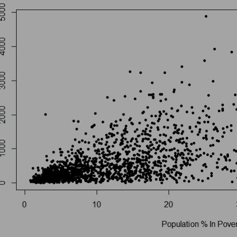
Covariance analysis reveals that many of the 123 potential independent predictors are correlated to each other. For example, a jurisdiction’s African American population percentage is correlated with its violent crime rate, as is the county’s poverty rate. Both predictors are also correlated with each other, presenting a multicolliniarity challenge in a typical linear regression.
A ridge regression is well suited to address this challenge with dozens of potential independent variables. A ridge regression was specified using the KNN classification algorithm, in addition to a basic KNN classification regression. Both were trained on normalized independent and dependent variables using a 10 fold cross-validation approach. The optimal ridge regression was determined based on R-squared performance.
CART Regression
Classification and Regression Trees (CART) models also address multicolliniarity through a decision tree approach, and is well suited for specifying significant independent variables from many options. Multiple CART models were specified and the model with the lowest cross-validation errors was chosen for pruning. The below decision tree shows the most important independent variable states from top to bottom, with terminal nodes that indicate average Violent Crime rates and the number of observations fitting within that node of the tree (n = #).

SVM Regression
Support Vectors Machines separates data points using hyperplanes to maximize the distance between clusters of observations. A SVM model was specified with a radial kernel, trained with a 10 fold cross-validation approach, and optimized based on R-squared performance.
Random Forest Regression
Random Forest is a decision tree model relying on both the bagging method of parallel training and feature selection randomness to generate multiple weak “tree” base learner models that are then aggregated into a “forest” model. The approach is considered “blackbox” in how challenging it is to externalize any interpretations, but the model can yield fantastic predictions when faced with many potential independent variables and highly variable data. A random forest model was trained on the entire predictor training dataset.
Predictions
To evaluate the performance of regression models root mean squared error (RMSE) and R-Squared were used. A model with a low RMSE and high R-Squared is desired. RMSE indicates the spread of the forecast errors. A model with high prediction volatility will have a higher RMSE value. R-Squared measures the correlation between the predicted values and the actuals in the validation set. The results for both for all six models are given in table 1 below.
The Random Forest model had the lowest RMSE and highest R-Squared values against the validation data. The CART model had the highest RMSE and lowest R-Squared value.
| Prediction Evaluators | Linear | GLM | KNN Ridge | KNN | CART | SVM | Random Forest |
|---|---|---|---|---|---|---|---|
| RMSE | 391.789 | 380.435 | 401.175 | 412.949 | 451.307 | 387.366 | 374.334 |
| R-Squared | 0.549 | 0.570 | 0.521 | 0.492 | 0.435 | 0.554 | 0.587 |
Discussion and Further Analysis
This analysis compares a linear regression model to machine learning models for predicting violent crime rates. Although the best performing model was the Random Forest model, the best linear regression model had a higher R-Squared value and lower RMSE than the worst three machine learning models: CART and both versions of the KNN algorithm. Interpretability and non-linear robustness is part of CART’s strong suits, but both it and KNN models are very susceptible to predictive variance depending on the makeup of the training dataset. Thirty-nine percent of the training observations ended up in one CART node, indicative of class imbalance that likely contributed to all three model’s shortcomings in prediction.
The underfitted CART node was on a branch for racially concentrated white, two parent household jurisdictions. Future analysis should consider if subsetting data for modeling in consideration of the effects of US segregation would improve CART’s predictive power.
To some extent an advantage of the linear regression model was its ability to control for some of the effects of racial concentration, likely through the inclusion of housing density. Model 3 has a more precise estimate of the white population percentage coefficient after estimating the independent relationship between housing density and violent crime rates.
GLM Boost and Random Forest regressions were the best performing models and both ensemble machine learning methods. Random Forest is different in its use of the bagging method which may have been well suited for a highly variant dataset with large outliers. Even GLM’s boosting clearly addressed some of the variation challenges posed by racially concentrated, household resourced jurisdictions.
This analysis was conducted in R. You can find the backup code and full variable list here, on my GitHub.